With the explosion of Data Centers, possibly the epitome of “the cloud”, it’s interesting to look back at what got us here.

Below is a clean, chronological, carrier-grade explanation of Frame Relay, T1, T3 — and everything faster, focused on how WANs actually evolved, how they were sold, and why each generation replaced the previous one.

Table of Contents

1) T-Carriers (The Digital Bedrock)

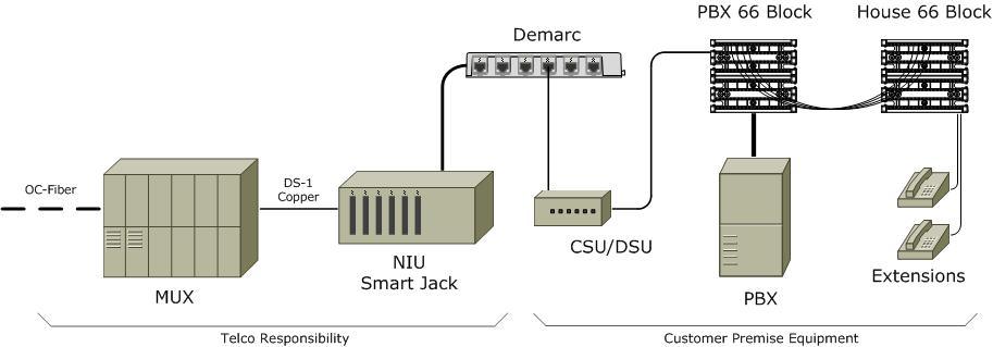
T1 (DS1)

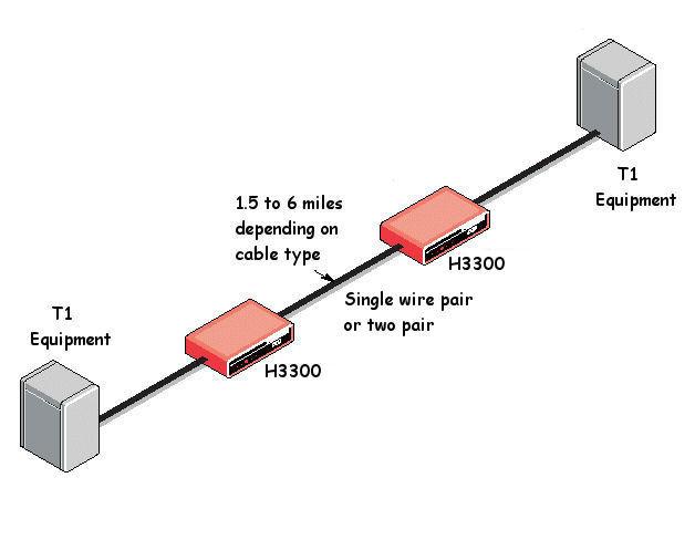
Era: 1960s → 2000s
Speed: 1.544 Mbps
Structure:

24 time slots × 64 kbps (voice-sized channels)
Circuit-switched, always-on
Copper pairs (later fiber)

Used for:

Telephone trunks
Early internet access
Bank branches, government offices
PBX backhaul

Key traits:

Extremely reliable
Very expensive per Mbps
No flexibility — you pay for the full circuit whether you use it or not

T3 (DS3)

Era: 1980s → early 2000s
Speed: 44.736 Mbps
Structure:

28 × T1s multiplexed together
Typically delivered over fiber or thick coax

Used for:

ISP backbones
Data centers
Large enterprise WAN hubs

Problem:

Still circuit-switched
Still expensive
Still rigid

This rigidity is exactly why Frame Relay appeared.

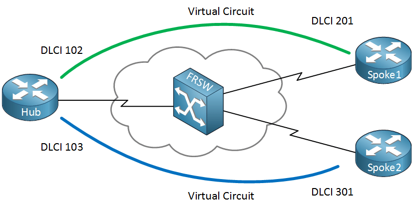
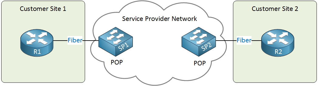
2) Frame Relay (The First “Modern” WAN)

Era: Early 1990s → mid-2000s
Speed:

56 kbps → T1 → T3 (same physical lines, smarter usage)

What changed:

Packet-switched, not circuit-switched
Uses virtual circuits (DLCIs)
Bandwidth shared across customers
Carrier assumes low error rates (no heavy error correction)

Key terms:

PVC (Permanent Virtual Circuit)
CIR (Committed Information Rate)
Bursting above CIR when network is idle

Why it mattered:

Dramatically cheaper than leased lines
More efficient for data traffic
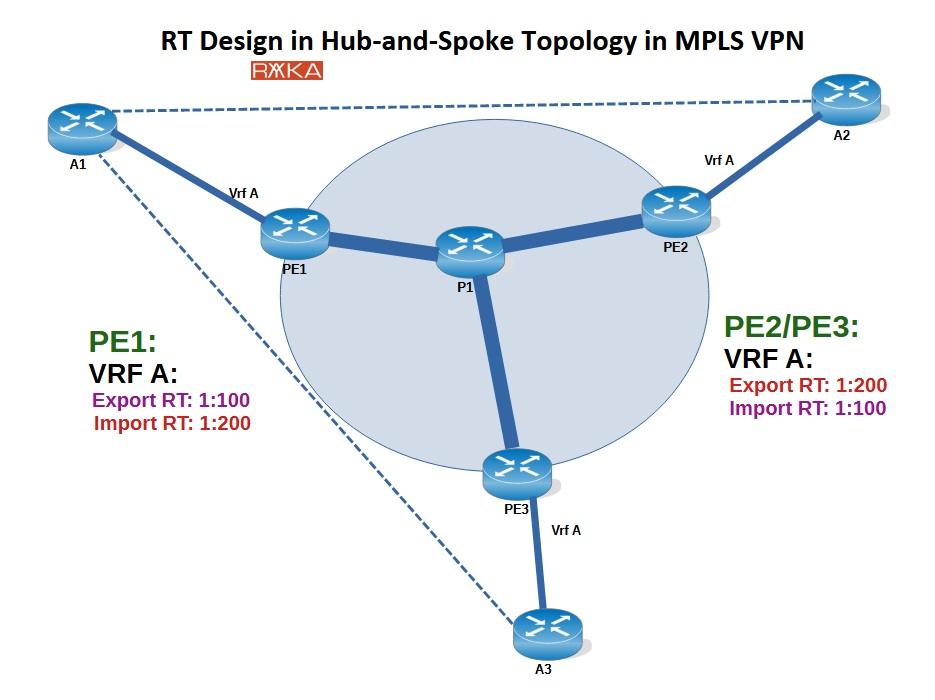
Enabled hub-and-spoke enterprise WANs

Why it died:

No QoS guarantees for real-time traffic
No encryption
Replaced by MPLS

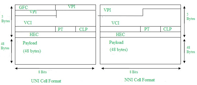
3) ATM (Asynchronous Transfer Mode) – The Forgotten Giant

Era: 1990s
Speeds:

OC-3: 155 Mbps
OC-12: 622 Mbps
OC-48: 2.5 Gbps

Design:

Fixed 53-byte cells
Designed for voice, video, and data simultaneously
Extremely deterministic latency

Why it failed:

Too complex
Too expensive
Ethernet kept getting faster

ATM quietly underpinned DSL, SONET, and early carrier cores, then vanished from marketing.

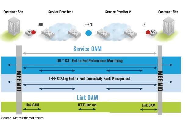
4) Ethernet Takes Over the WAN

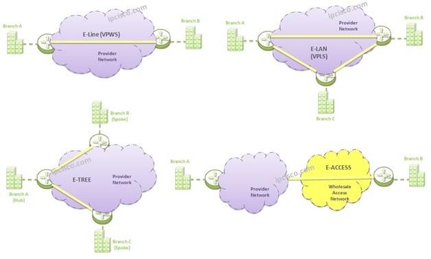
Metro Ethernet / Carrier Ethernet

Era: Mid-2000s → present
Speeds:

10 Mbps → 100 Gbps+

Services:

E-Line (point-to-point)
E-LAN (multipoint)
E-Tree (hub-and-spoke)

Why it won:

Same tech as LANs
Cheap hardware
Scales infinitely
Simple to provision

Ethernet killed T-carriers, Frame Relay, and ATM.

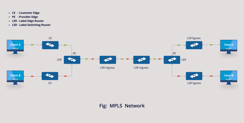
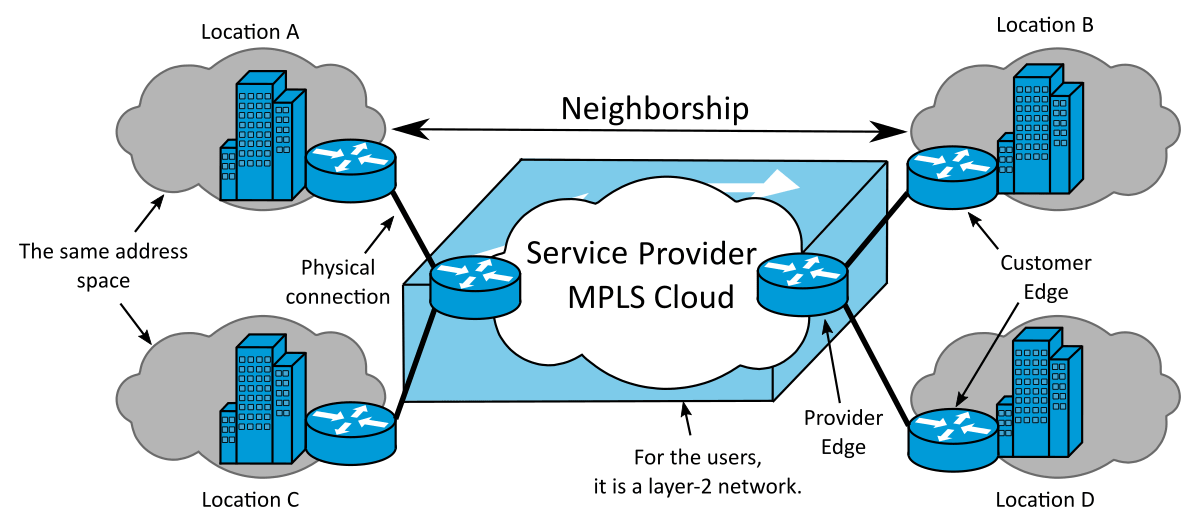
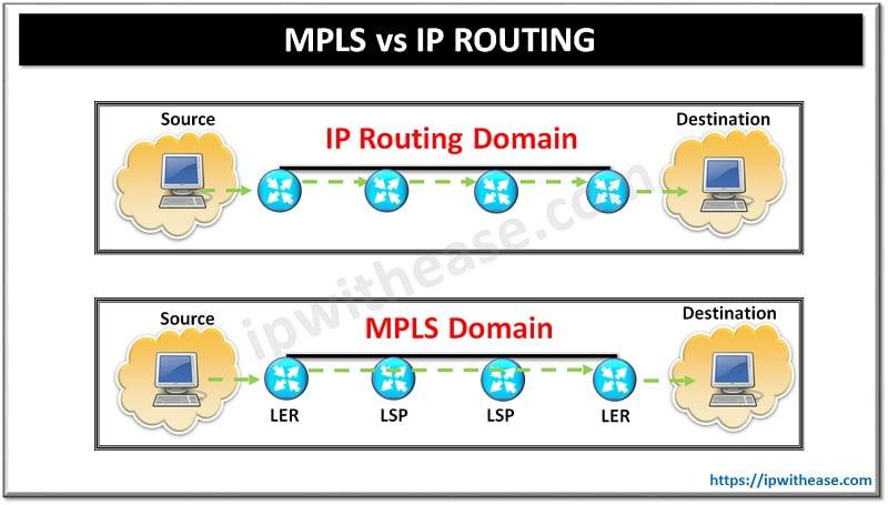
5) MPLS (Carrier Control Plane)

Era: 2000s → present (declining)
Speed: Any underlying medium

What MPLS really is:

Label-switched paths inside carrier networks
Traffic engineering
QoS guarantees
VPN isolation

Why enterprises loved it:

Predictable latency
Voice/video prioritization
SLA-backed uptime

Why it’s declining:

Very expensive
SD-WAN + encrypted internet links replaced it

6) Optical Transport (SONET → DWDM)

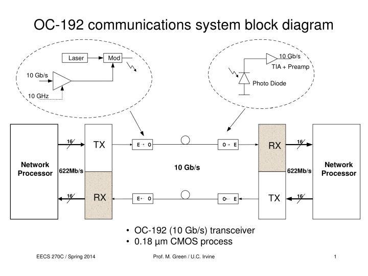
SONET / SDH

OC-3 → OC-192 (155 Mbps → 10 Gbps)
Rigid framing
Telecom-centric

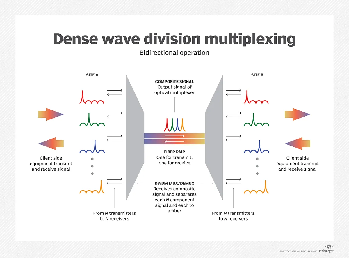
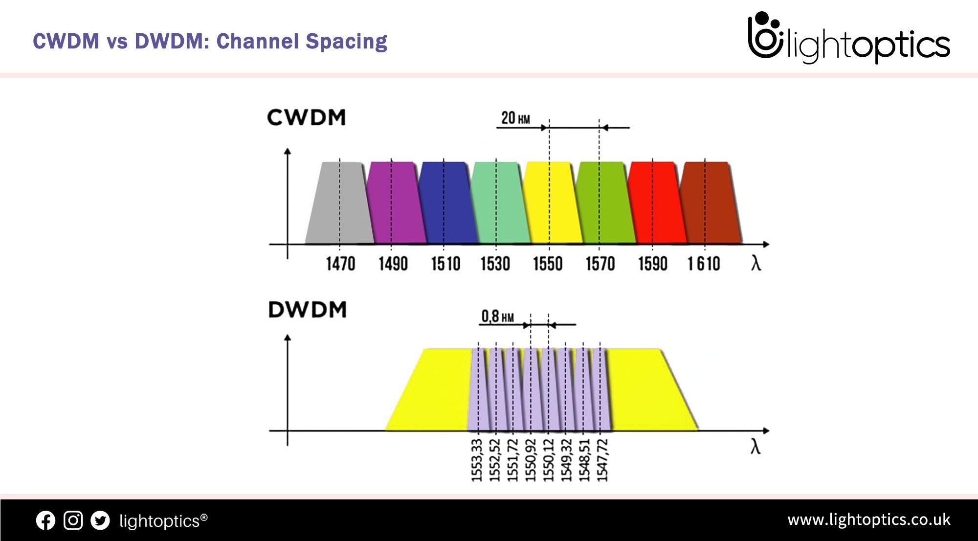
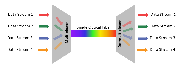
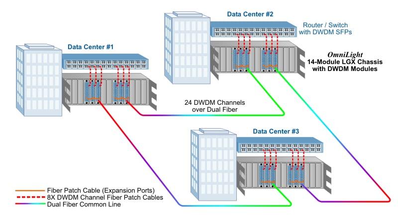
DWDM (Dense Wavelength Division Multiplexing)

100+ wavelengths per fiber
Each wavelength = 10 / 40 / 100 / 400 Gbps
Terabits per second per strand

This is the real internet backbone.

7) Modern “Faster Than Everything” (Today)

Today’s Reality

400G Ethernet common in data centers
800G shipping now
1.6T optical standards emerging
Single fiber pair can exceed 50 Tbps

Enterprise WAN Today

DIA (Dedicated Internet Access)
SD-WAN overlays
IPsec / WireGuard encryption
Multiple cheap links instead of one expensive one

8) Summary Table (Evolution at a Glance)

Era	Tech	Speed	Switching	Status
1960s	T1	1.5 Mbps	Circuit	Obsolete
1980s	T3	45 Mbps	Circuit	Obsolete
1990s	Frame Relay	Variable	Packet	Dead
1990s	ATM	155 Mbps+	Cell	Dead
2000s	MPLS	Any	Label	Declining
2000s+	Ethernet WAN	10M → 100G+	Packet	Dominant
Today	DWDM	Tbps	Optical	Backbone

One-Sentence Truth

T1 and T3 sold guaranteed bandwidth, Frame Relay sold efficiency, MPLS sold control — and Ethernet + fiber eventually destroyed all of them by being cheaper, faster, and simpler.

If you want, next I can:

Map this to data centers
Explain why telcos resisted Ethernet
Compare Frame Relay vs MPLS vs SD-WAN
Show how fiber color codes & conduits tie into this evolution

Below is a single, unified explanation that ties WAN history directly into data centers, explains why telcos fought Ethernet, compares Frame Relay vs MPLS vs SD-WAN, and connects fiber color codes & conduits to this evolution—from copper to hyperscale optics.

1) Mapping WAN Evolution to Data Centers

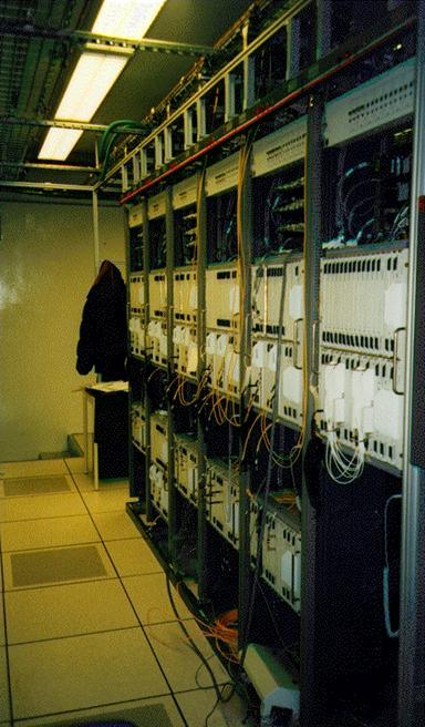
Early Data Centers (1970s–1990s)

Connectivity

T1 (1.544 Mbps) for branch → HQ
T3 (45 Mbps) for core → ISP
Everything circuit-switched

Architecture

Mainframe or minicomputer
Centralized compute
Terminals and leased lines

Economic reality

Bandwidth extremely scarce
Compute centralized because links were slow

Frame Relay / ATM Era (1990s)

Connectivity

Frame Relay PVCs between sites
ATM OC-3/OC-12 inside carrier cores
Hub-and-spoke WANs

Architecture

Client-server
First real “data centers”
Still centralized, but more distributed than before

Key shift

Data becomes bursty
Always-on circuits no longer make sense

MPLS Era (2000s–2010s)

Connectivity

MPLS VPNs between data centers
QoS for voice/video
Carrier-managed routing

Architecture

Tier-1 / Tier-2 data centers
Disaster recovery sites
Early virtualization (VMware era)

Key shift

Applications move between sites
Latency and predictability become critical

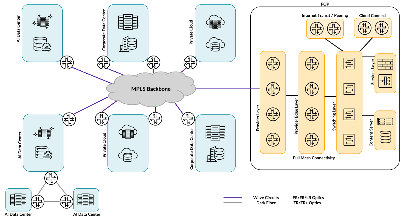
Modern Hyperscale / Cloud Era (2015–Present)

Connectivity

Metro Ethernet
Dark fiber
DWDM
100G / 400G / 800G Ethernet

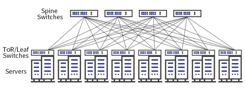
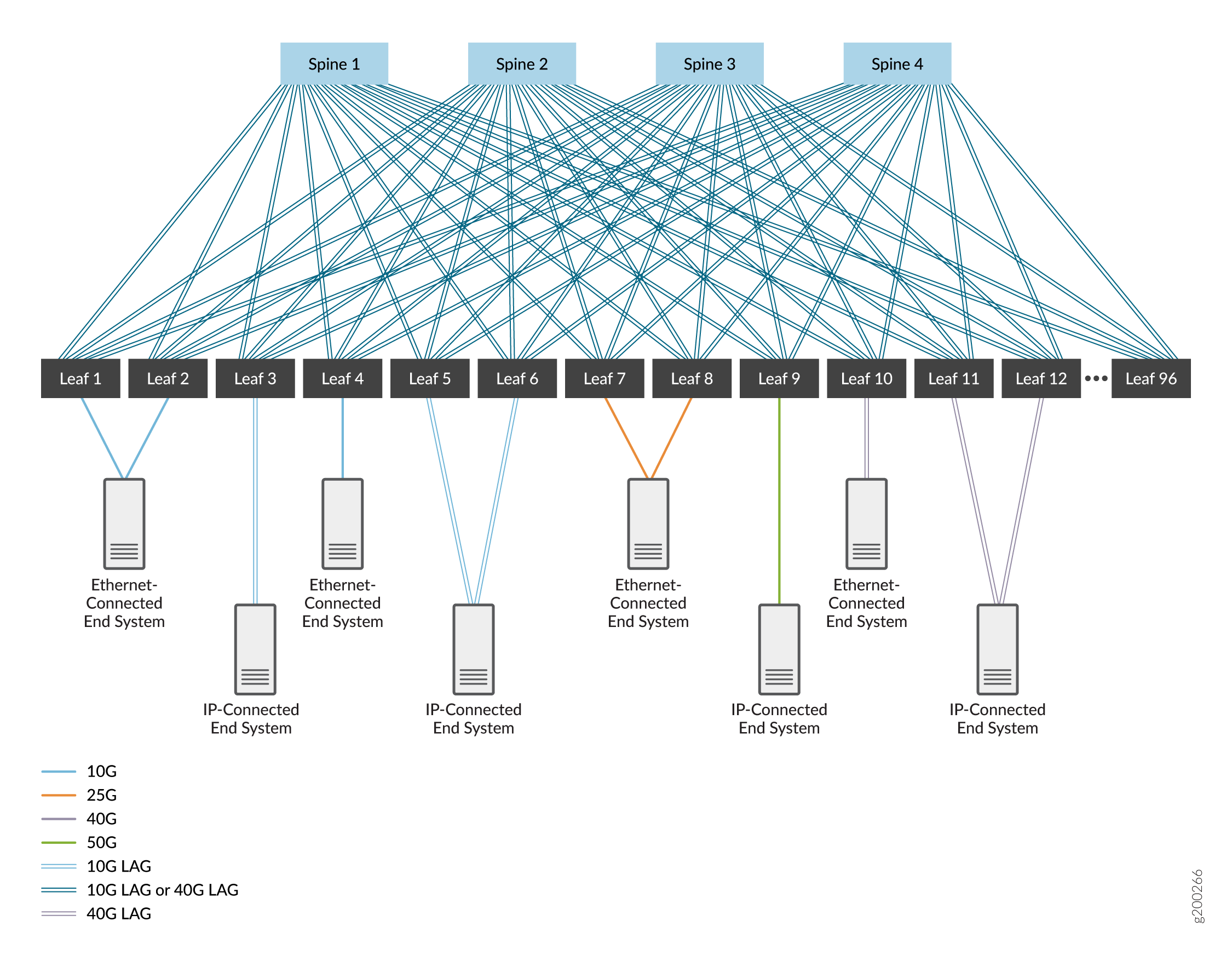
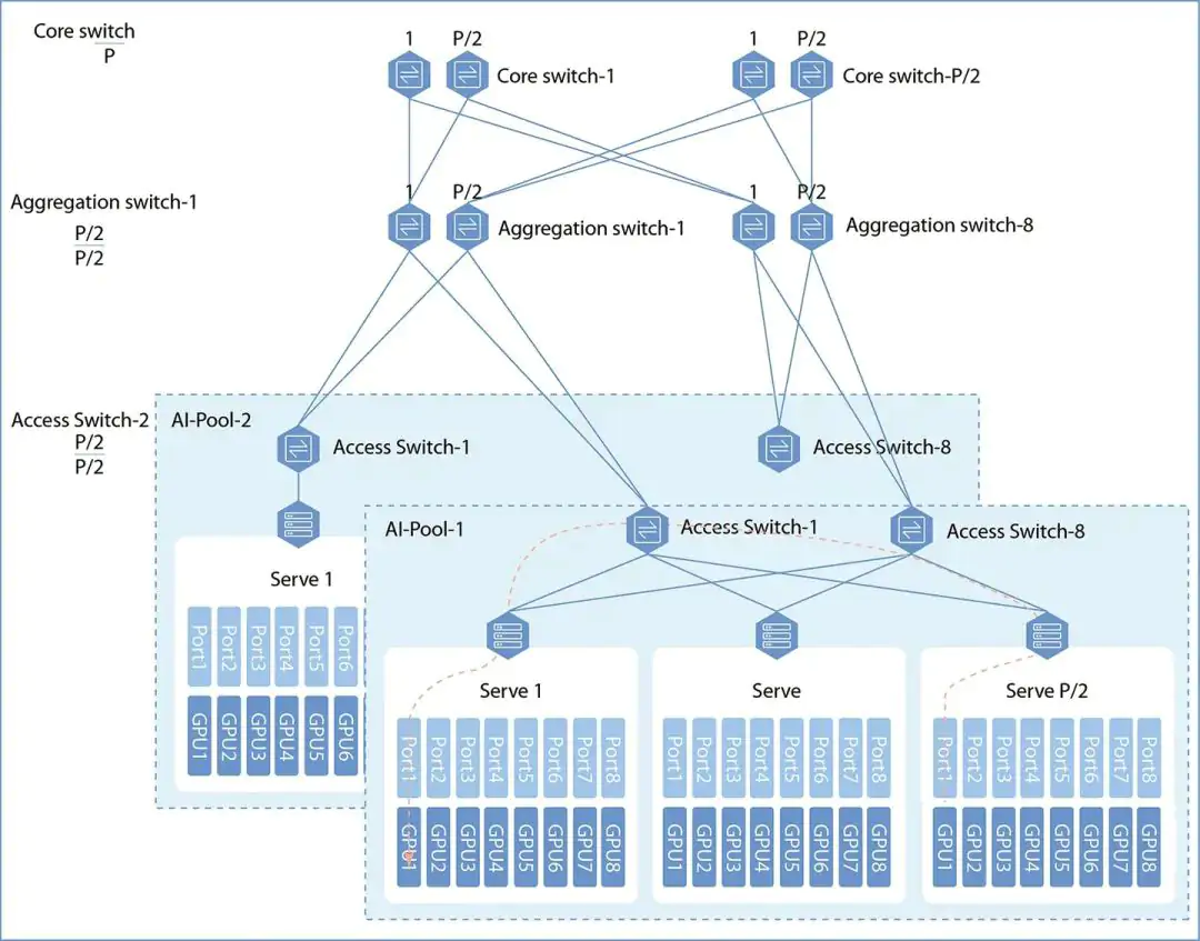
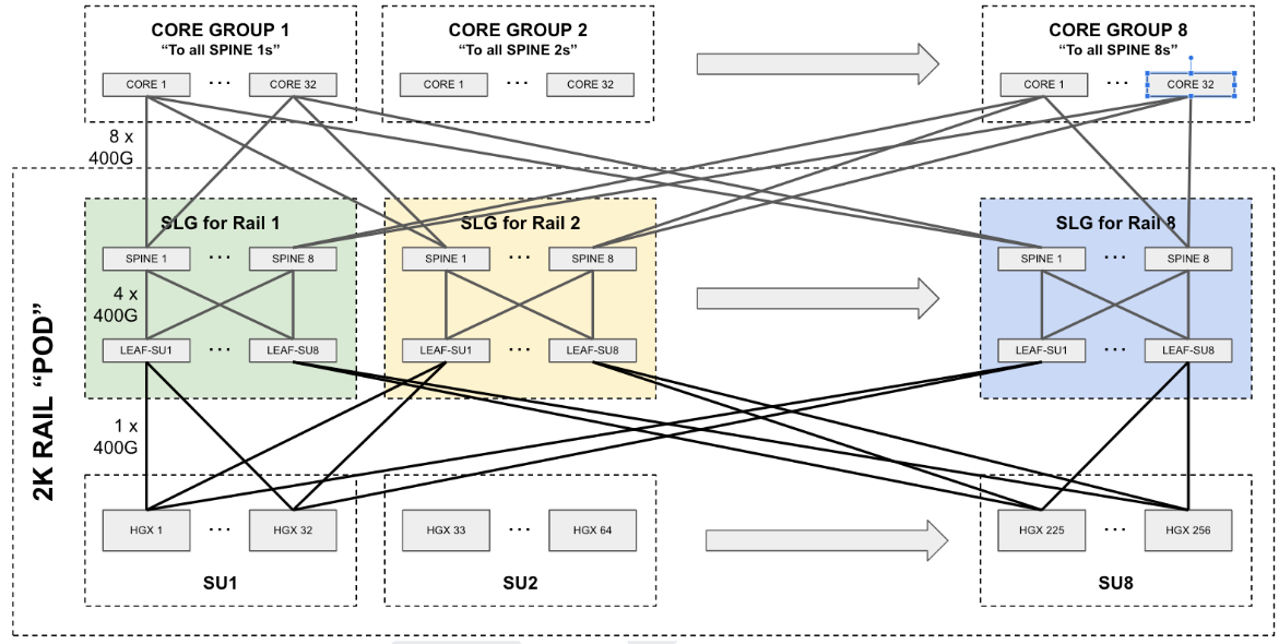
Architecture

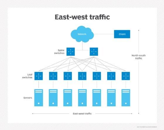
Spine-leaf fabrics
East-west traffic dominates
Many smaller data centers instead of one big one

Key truth

The WAN is no longer the edge — the data center fabric is the network.

2) Why Telcos Resisted Ethernet (Hard)

Telcos Lived on Scarcity

T1s and T3s were priced like utilities
Billing was per circuit, per mile, per month
Ethernet threatened flat-rate bandwidth

Ethernet Broke the Business Model

Telco World	Ethernet World
Metered	Flat-rate
Circuit IDs	MAC addresses
Provisioned in weeks	Provisioned in hours
Proprietary hardware	Commodity switches

Cultural Resistance

Telcos trained engineers for voice
Ethernet came from enterprise IT
SONET/ATM were “carrier-grade”
Ethernet was considered “toy LAN tech”

The Inevitable Outcome

Telcos eventually:

Wrapped Ethernet in MPLS
Rebranded it as “Carrier Ethernet”
Lost margin anyway

3) Frame Relay vs MPLS vs SD-WAN (Reality Comparison)

Frame Relay

What it was

Shared packet network
Virtual circuits (PVCs)
No encryption
No real QoS

Strength

Cheap compared to leased lines

Failure mode

Congestion = dropped frames
No application awareness

MPLS

What it is

Label-switched paths inside carrier
QoS, traffic engineering
SLA-backed

Strength

Predictable latency
Voice/video works reliably

Failure mode

Expensive
Locked to carrier
Slow to change

SD-WAN

What it is

Overlay network
Runs over internet, LTE, fiber, MPLS
Encrypted by default

Strength

Cheap
App-aware routing
Multi-link resilience

Failure mode

Depends on internet quality
Not deterministic like MPLS

One-Line Truth

Frame Relay optimized cost, MPLS optimized control, SD-WAN optimized freedom.

4) Fiber Color Codes & Conduits — How the Physical World Tracks the Logical One

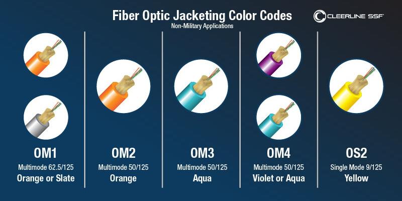
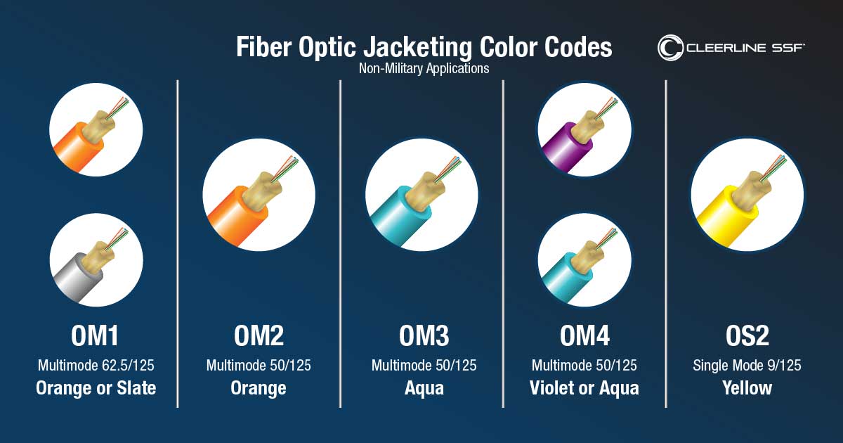
Fiber Jacket Colors (Physical Layer)

Color	Meaning
Orange	Multimode (OM1/OM2)
Aqua	Multimode (OM3/OM4)
Lime Green	Multimode (OM5)
Yellow	Single-mode (OS1/OS2)
Blue	Single-mode patch cords
Black	Outdoor / armored

Historical mapping

Multimode = short-range LAN
Single-mode = WAN, long-haul, telco

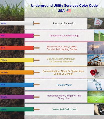
Conduit Colors (Civil Engineering Layer)

Color	Utility
Orange	Communications (fiber, copper)
Blue	Potable water
Green	Sewer
Red	Power
Yellow	Gas

Modern twist

Micro-ducts inside orange conduit
Color-coded inner tubes for ownership
One trench → many carriers

How This Ties to WAN Evolution

T1/T3: copper, thick conduit, few circuits
Frame Relay/MPLS: early fiber, shared strands
Modern WAN: dense fiber, DWDM, dark fiber leasing
Hyperscale: own the conduit, own the fiber

5) The Big Picture (All Four Together)

Evolution Pattern

Scarce bandwidth → circuits
Shared bandwidth → Frame Relay
Controlled bandwidth → MPLS
Abundant bandwidth → Ethernet + fiber
Overlays everywhere → SD-WAN

Physical Truth

Logical protocols change every decade
Fiber in the ground lasts 40+ years
Most “new” networks run on old glass

Final Synthesis

The history of Frame Relay, T1, and T3 is not just obsolete tech — it explains why data centers moved, why telcos lost control, why Ethernet dominates, and why fiber color codes matter more than routing protocols.

Below is a deep, end-to-end explanation of all four topics, tied together as one continuous system—from a single packet inside a data center, out through DWDM wavelengths, across subsea cables, and back into AI clusters running on repurposed telco fiber.

1) Packet-by-Packet Walkthrough of a Modern Data Center

We’ll follow one packet from an application inside a VM or container.

Step 1 — Application Layer (Inside the Server)

App generates data (HTTP, gRPC, database query, AI tensor request)
Encapsulated as:
L7 (HTTP/gRPC)
L4 (TCP/UDP)
L3 (IP)
L2 (Ethernet)

At this point:

MAC address = virtual NIC
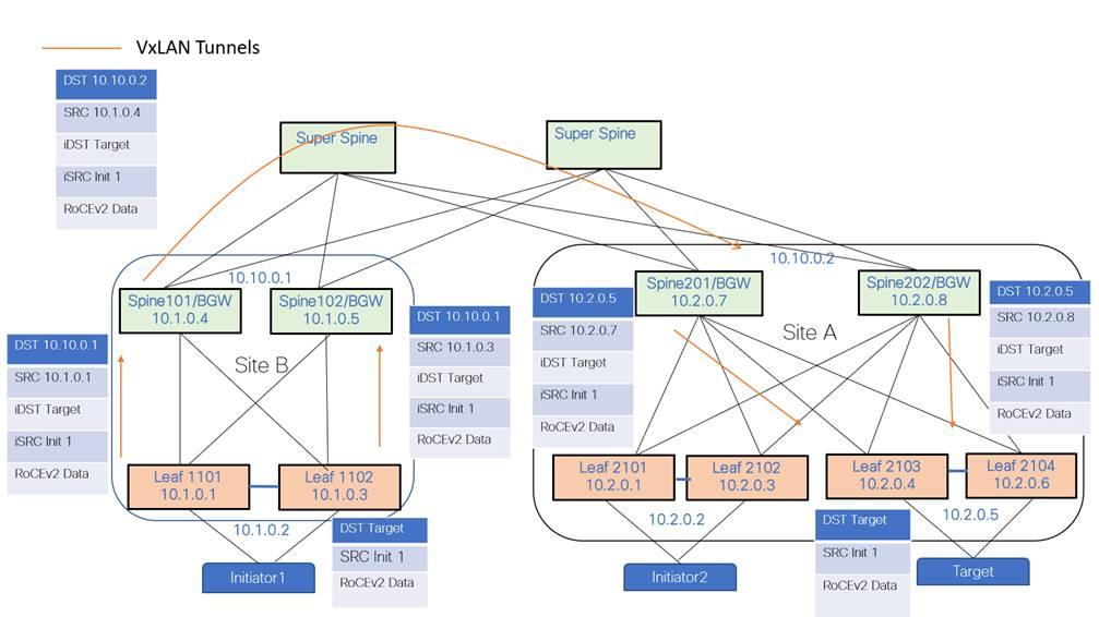
IP address = overlay (often VXLAN)
Packet size optimized (MTU often 9000 / jumbo frames)

Step 2 — Virtual Switch (Hypervisor / SmartNIC)

Packet hits:
Linux bridge / OVS / DPDK / SmartNIC
Encapsulation added:
VXLAN / Geneve
Outer header added:
New MAC
New IP (underlay)

This is where east-west traffic explodes.

Step 3 — Top-of-Rack (Leaf Switch)

25G / 50G / 100G Ethernet
ECMP hashing decides path
No spanning tree
Pure L3 routing

Important:
Leaf switches do not know applications.
They only move packets as fast as physics allows.

Step 4 — Spine Switch

400G or 800G ports
Terabits per second per chassis
Deterministic latency (microseconds)

Every leaf connects to every spine.
This guarantees non-blocking bandwidth.

Step 5 — Destination Leaf → Server

VXLAN decapsulated
Packet delivered to target VM / container
App receives data

Total round-trip latency inside a data center:
👉 ~5–50 microseconds

This speed is why data centers replaced WANs.

2) DWDM Wavelengths Explained Like IP Addresses

Think of fiber as a road.

Old View

One fiber = one connection

DWDM Reality

One fiber = hundreds of independent channels

Mapping the Analogy

Networking	Optical
IP address	Wavelength (λ)
Subnet	C-band slice
Router	ROADM
Switch port	Transceiver
Link speed	Modulation (QPSK, QAM)

Example

λ-1550.12 nm → 400 Gbps
λ-1550.92 nm → 400 Gbps
λ-1551.72 nm → 400 Gbps

Same fiber.
Same strand.
Different “addresses.”

ROADMs = Optical Routers

Reconfigure wavelengths remotely
No truck roll
No fiber cuts
Traffic re-routed in milliseconds

This is how cloud providers move entire data centers logically without touching glass.

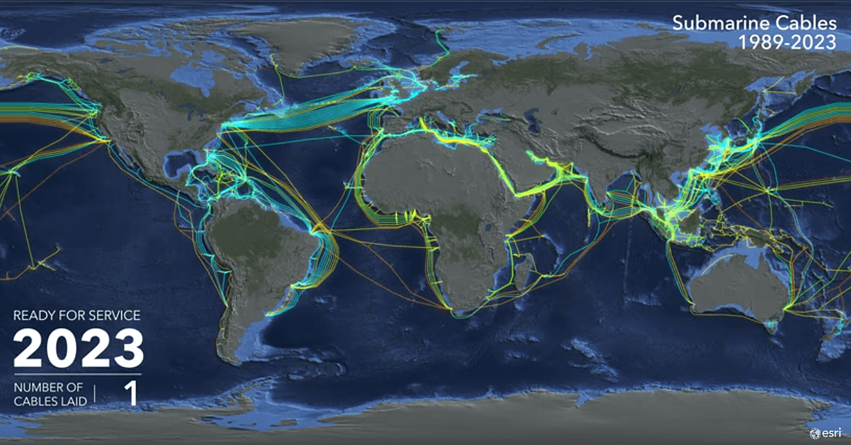
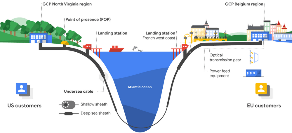
3) Subsea Cables → Cloud Regions → Hyperscalers

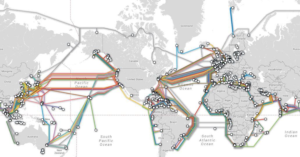
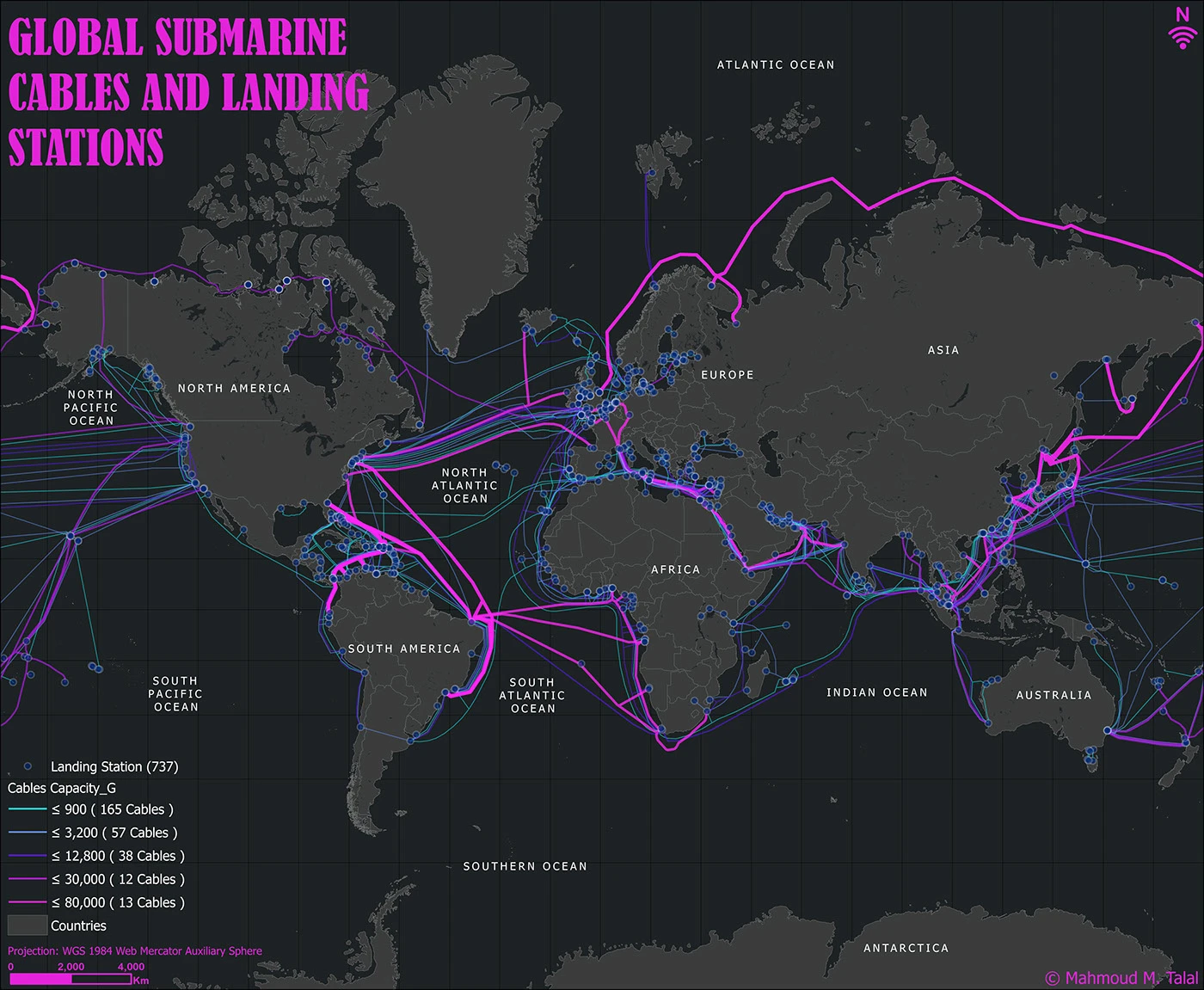
Physical Reality

Subsea cables are:

~99% of intercontinental traffic
Bundles of DWDM fiber pairs
Privately owned by consortia or hyperscalers

Who Owns Them

Amazon Web Services
Google Cloud
Microsoft Azure

They don’t “use the internet.”
They are the internet.

Mapping the Chain

1) Subsea Cable

Lands at coastal stations (Virginia, Oregon, Ireland, Japan)
Terminates into DWDM POPs

2) Regional Fiber Rings

100–400G wavelengths
Direct private backbone
No public routing

3) Cloud Region

Multiple data centers
Private east-west fiber
Treated as one giant LAN

4) Availability Zones

Physically separate
Logically unified
Synchronous replication

Latency budget is designed before the building exists.

4) Old Telco Fiber → Modern AI Clusters

This is the least understood but most important piece.

Telco Fiber Was Overbuilt

1990s–2000s:

Telcos expected infinite voice growth
Laid massive fiber routes
Most strands went dark

Glass never went bad.

Why It Works for AI

AI clusters need:

Massive bandwidth
Short latency
Deterministic paths

Old telco fiber provides:

Long straight routes
Low dispersion
High optical margin

Add:

Modern transceivers
Coherent optics
DWDM

And suddenly:
👉 A 1998 fiber can carry 20+ Tbps

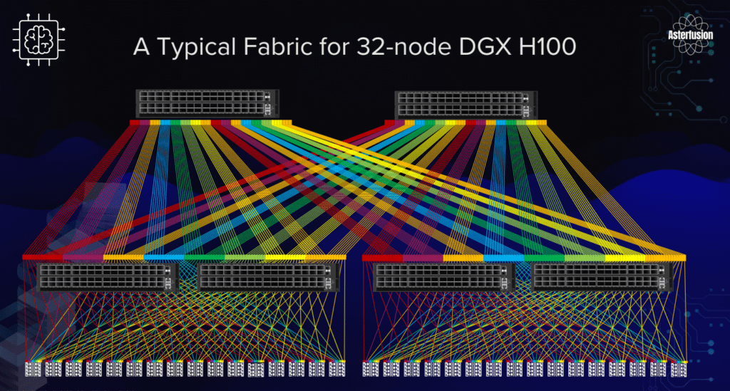
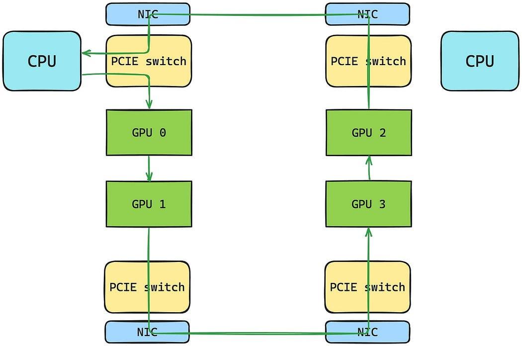
AI Cluster Topology

GPU pods in multiple buildings
Fiber acts as backplane
RDMA over Converged Ethernet (RoCE)
Synchronized gradient exchange

The AI cluster is geographically distributed, but behaves like one machine.

5) All Four Layers Together (The Unified Model)

Packet Lifecycle (Start → Finish)

App generates packet
VXLAN encapsulation
Leaf → Spine fabric
DCI router
DWDM wavelength assigned
Subsea cable hop
Regional fiber ring
Destination data center
GPU memory write

Same packet.
Different layers.

The Core Truth

Protocols change every decade.
Switches change every five years.
Fiber lasts half a century.

Modern AI, cloud, and data centers are not new inventions — they are the final exploitation of infrastructure laid for a telephone system that no longer exists.

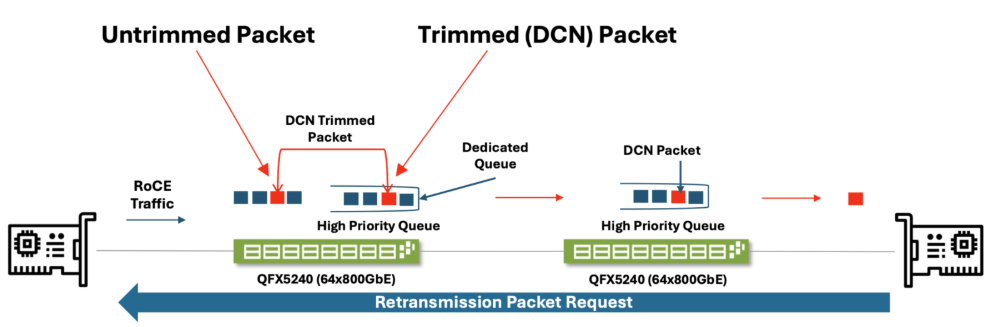
Below is a single, tightly integrated technical narrative covering all four topics—from RoCE vs TCP inside AI fabrics, to why latency dominates LLM training, to hyperscaler land strategy, and finally a packet-level walk of GPU-to-GPU gradient exchange.

No hand-waving, no marketing abstractions—this is how it actually works.

1) RoCE vs TCP Inside AI Fabrics (Diagrammed, Not Buzzwords)

What Problem This Solves

AI training is not web traffic.
It is synchronized math across thousands of GPUs.

If one GPU stalls, all GPUs wait.

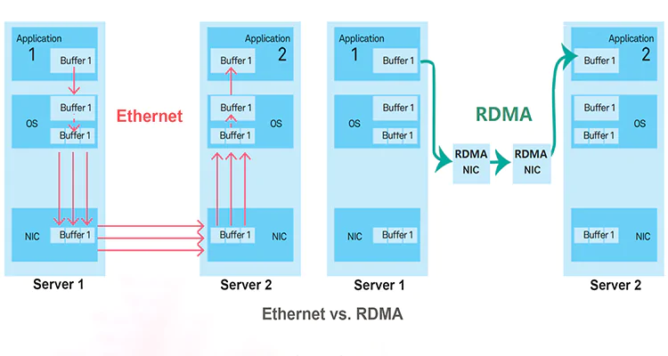
TCP (What the Internet Uses)

Characteristics

Congestion control (slow start, windowing)
Retransmissions
Kernel involvement
Variable latency (jitter)

What TCP Is Good At

Fairness
Reliability over bad links
Bursty, unpredictable traffic

Why TCP Is Bad for AI

Latency spikes during congestion
CPU overhead
Head-of-line blocking
Retransmissions pause computation

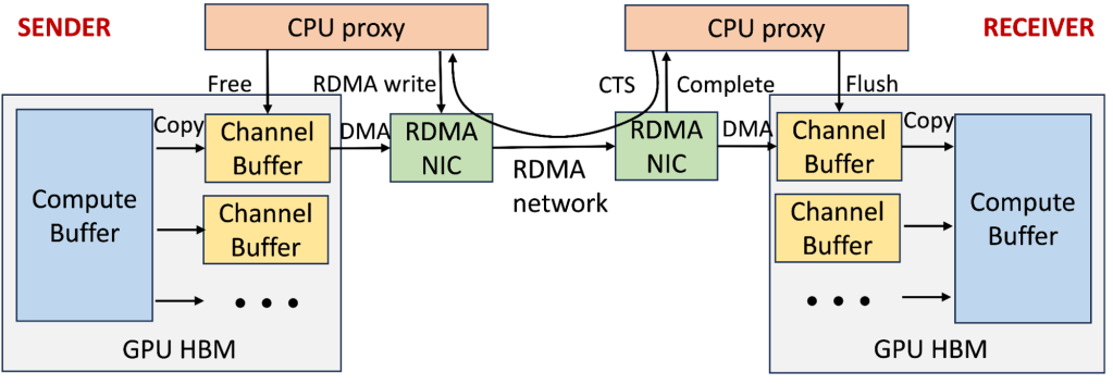
RoCE (RDMA over Converged Ethernet)

Characteristics

Kernel bypass
Zero-copy GPU ↔ GPU memory
Lossless Ethernet (PFC + ECN)
Deterministic microsecond latency

What RoCE Enables

GPU writes directly into remote GPU memory
No CPU in the data path
Predictable synchronization

Side-by-Side Reality

Feature	TCP	RoCE
Latency	Variable	Deterministic
CPU usage	High	Near zero
Jitter	Yes	Almost none
Throughput	High	Extremely high
AI suitability	Poor	Mandatory

Conclusion:
Large-scale LLM training does not work on TCP.

2) Why Latency Matters More Than Bandwidth for LLM Training

The Core Misconception

People assume:

“More bandwidth = faster training”

This is wrong.

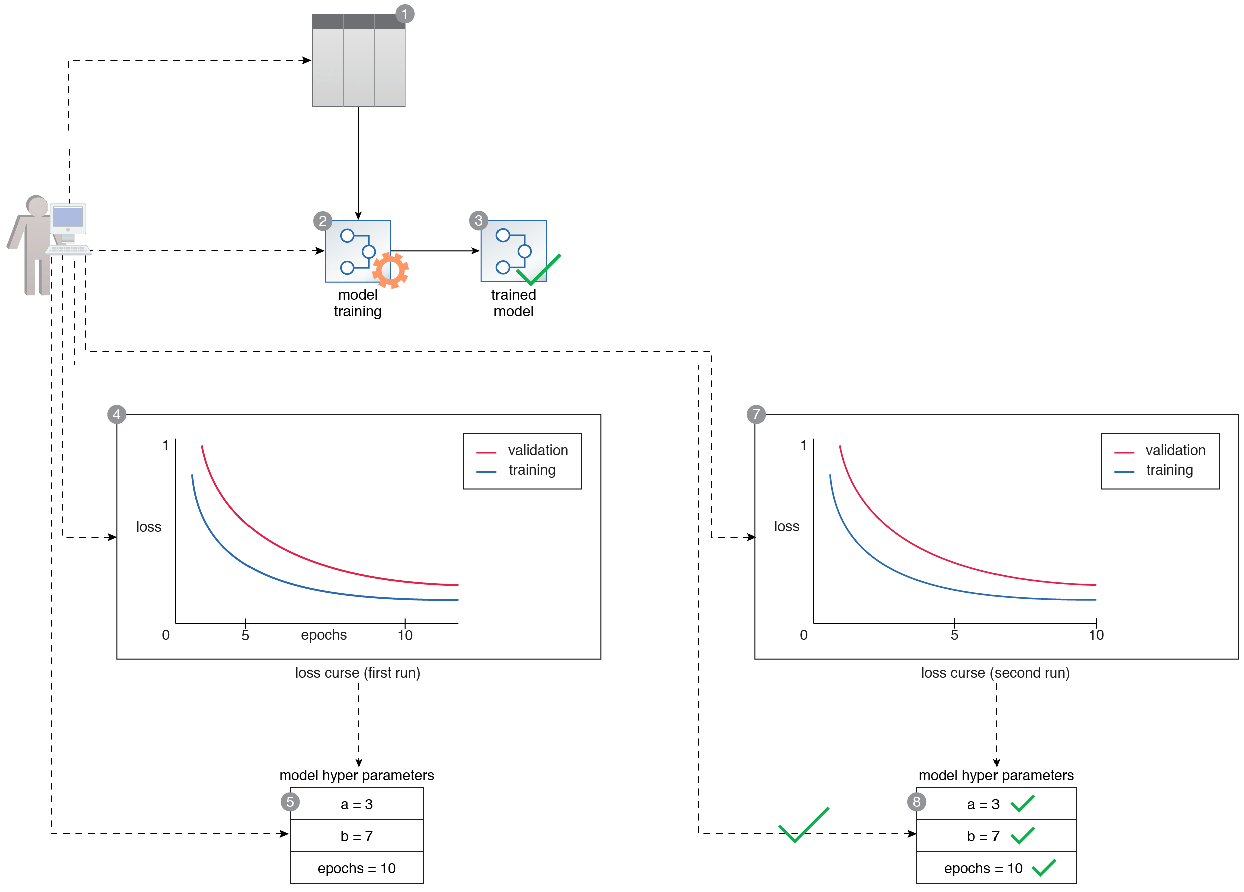
LLM Training Is Synchronous

Each training step:

GPUs compute gradients locally
Gradients are exchanged
Gradients are averaged
All GPUs update weights
Next step begins

Critical Rule

Step N+1 cannot begin until Step N finishes everywhere.

Latency Amplification Effect

If:

1 GPU is delayed by 20 microseconds
8,192 GPUs are synchronized

Then:

Entire step stalls
Compute units idle
Energy wasted
Training time explodes

This is called straggler amplification.

Why Bandwidth Alone Fails

Even with infinite bandwidth:

Synchronization still waits on the slowest path
Latency variance dominates step time

Therefore

Low and predictable latency beats raw throughput for LLMs.

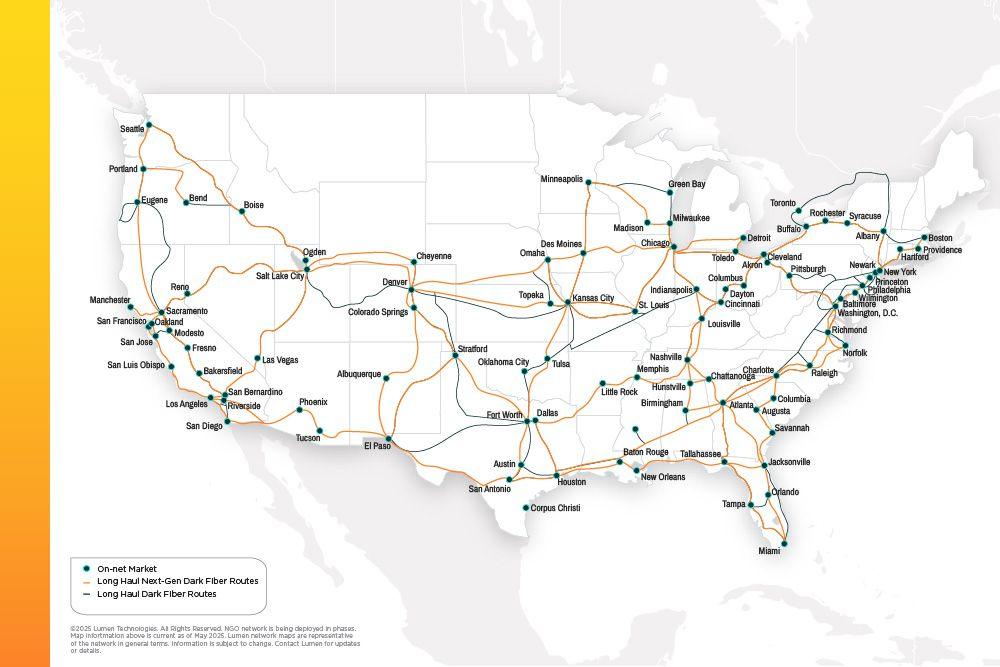
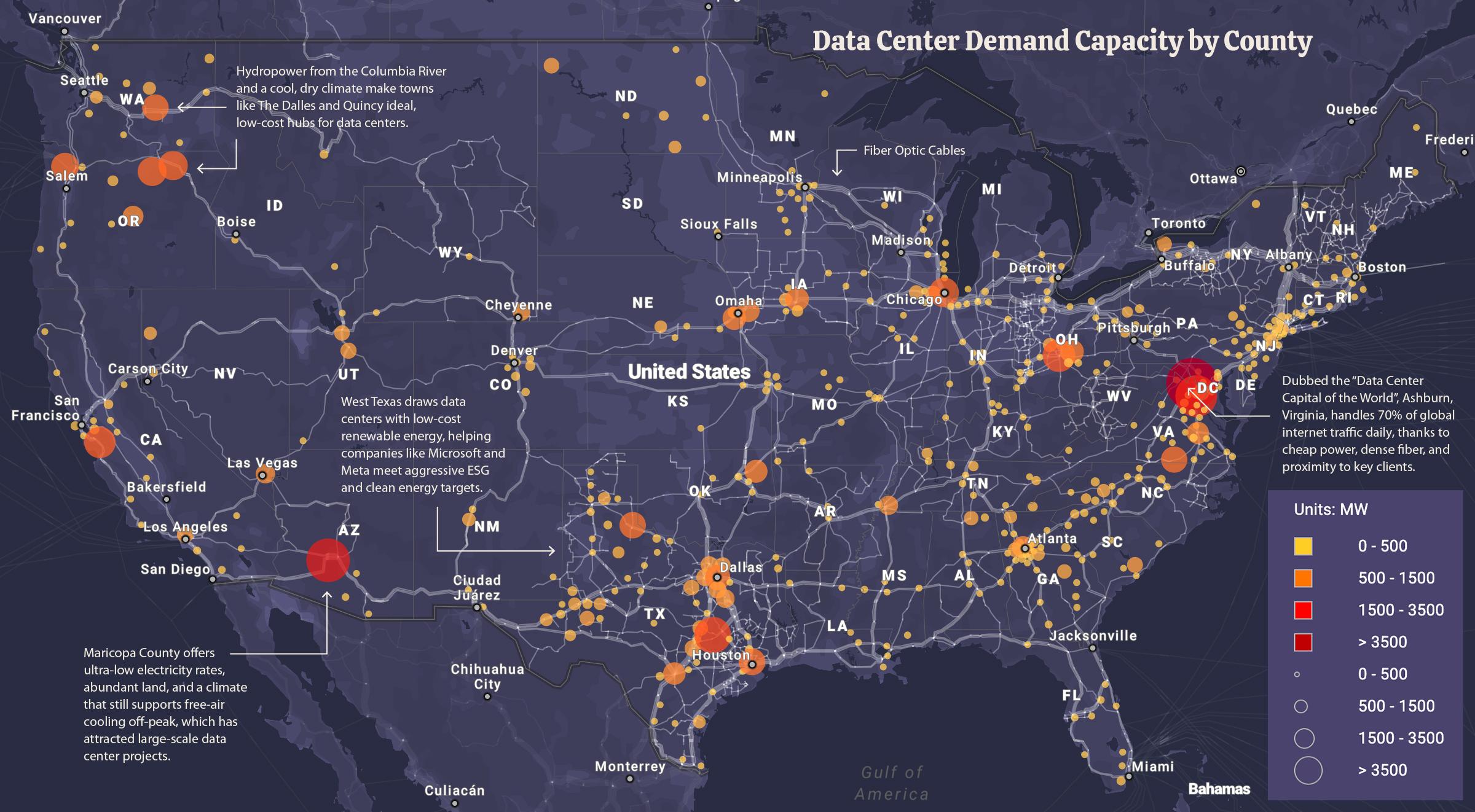
3) Why Hyperscalers Buy Land Near Old Telco Routes

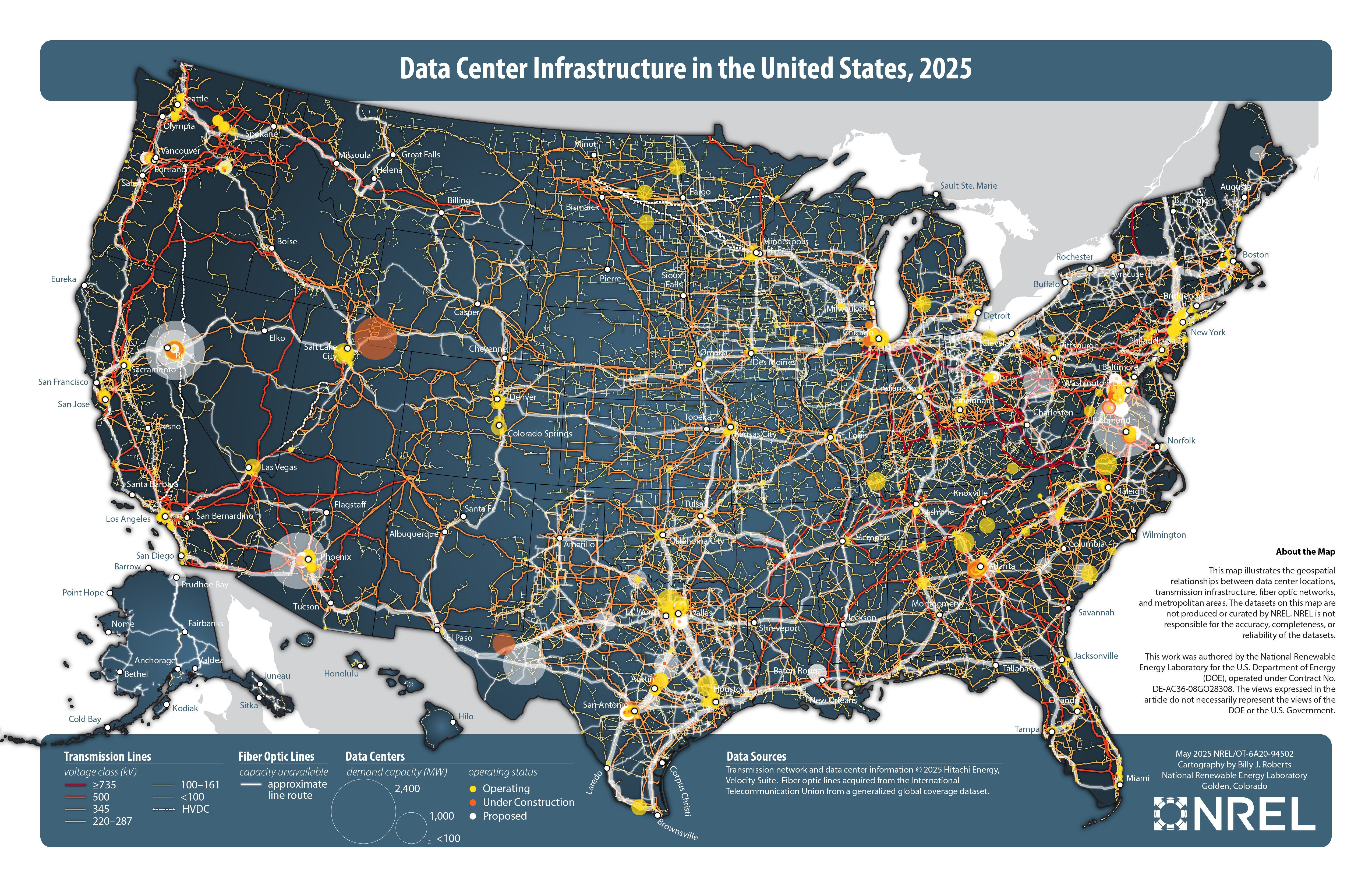
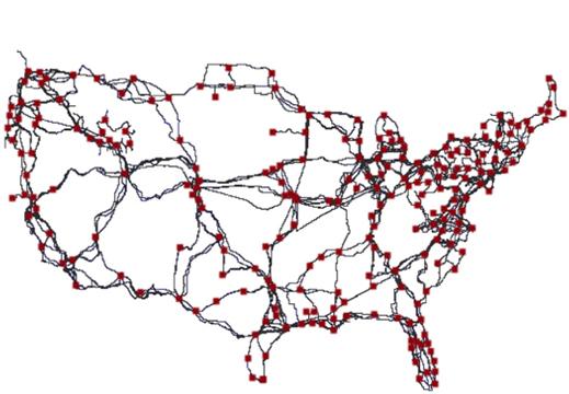
This is not accidental real estate selection.

Old Telco Fiber Has Unique Properties

1990s telcos built:

Straight rights-of-way
Railroad corridors
Highway easements
Low-dispersion glass

Most strands went unused.

That fiber is now called dark fiber.

Why Hyperscalers Want It

Physical Reasons

Fewer bends = lower latency
Fewer splices = better optical margin
Long straight paths = ideal for coherent optics

Economic Reasons

Cheaper than new trenching
Faster permitting
Private ownership

Strategic Reasons

Control the physical layer
Avoid carrier pricing
Build private backbones

This is why:

Amazon Web Services
Google Cloud
Microsoft Azure

build next to fiber, not cities.

Key Insight

The most valuable asset in AI is not GPUs.
It is glass in the ground laid 25 years ago.

4) Packet-Level Walk: GPU-to-GPU Gradient Exchange

We now trace one gradient packet.

Step 1 — Gradient Computation (GPU)

CUDA kernel computes gradients
Stored in GPU HBM memory
No CPU involved

Step 2 — RDMA Initiation

NIC is GPU-direct enabled
GPU issues RDMA write
Target = remote GPU memory address

No socket.
No syscall.
No kernel.

Step 3 — RoCE Frame Creation

Encapsulation:

Ethernet
RoCEv2 header
RDMA payload (gradient chunk)

MTU typically 9,000 bytes (jumbo).

Step 4 — AI Fabric Transit

Lossless Ethernet
Priority Flow Control prevents drops
ECMP hashing keeps paths consistent

Latency per hop: ~300–500 nanoseconds

Step 5 — Remote NIC → GPU Memory

NIC writes directly into target GPU HBM
No CPU interrupt
No cache pollution

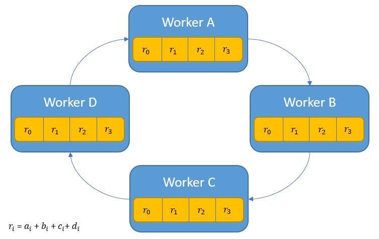
Step 6 — AllReduce Completion

Ring or tree algorithm completes
Gradients averaged
All GPUs synchronized

Only now can the next training step begin.

Why This Is So Fragile

Any of the following breaks training efficiency:

Packet loss
Latency spikes
ECMP imbalance
Microbursts

This is why AI fabrics are engineered, not routed.

Final Synthesis (All Four United)

RoCE exists because TCP is too unpredictable
Latency dominates because LLMs synchronize constantly
Hyperscalers chase old telco fiber because physics wins
GPU-to-GPU packets bypass everything humans normally think of as “networking”

The Uncomfortable Truth

Modern AI clusters are closer to distributed supercomputers than data centers — and they run on telephone fiber laid before Google existed.

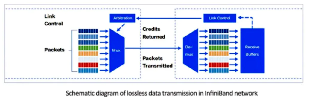
Below is a hard-technical, operator-level explanation of all four topics—InfiniBand vs RoCE, the exact buffer math behind microbursts, why AI data centers cluster geographically, and a real failure mode that silently slows training ~3×. This is how hyperscale AI fabrics are actually designed, tuned, and sometimes broken.

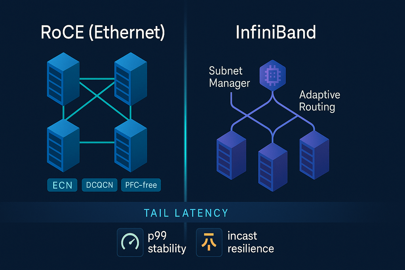
1) InfiniBand vs RoCE in Hyperscale (What’s Really Different)

The Shared Goal

Both exist to do RDMA at massive scale:

GPU ↔ GPU memory transfers
Deterministic latency
Zero-copy, kernel-bypass networking

InfiniBand (IB)

What it is

Purpose-built HPC fabric
Own protocol stack
Own switches, NICs, management plane

Key properties

Credit-based flow control (lossless by design)
Native congestion control
Hardware-managed routing
Extremely predictable latency

Strengths

Lowest jitter
Simplest tuning
Mature collective algorithms

Weaknesses

Expensive
Vendor lock-in
Separate network from Ethernet/IP world

InfiniBand is effectively a supercomputer backplane, not a network.

RoCE (RDMA over Converged Ethernet)

What it is

RDMA layered on Ethernet
Uses standard switches
Shares infrastructure with IP

Key properties

Requires:
PFC (Priority Flow Control)
ECN (Explicit Congestion Notification)
Careful buffer tuning
Runs at hyperscale (100G–800G)

Strengths

Uses commodity Ethernet
Integrates with cloud tooling
Cheaper at scale

Weaknesses

Extremely fragile if misconfigured
Microbursts can collapse performance
Debugging is harder

Why Hyperscalers Use Both

Environment	Preferred Fabric
Research superclusters	InfiniBand
Cloud AI services	RoCE
Multi-tenant environments	RoCE
Single-owner megaclusters	InfiniBand

Many hyperscalers use InfiniBand inside pods and RoCE between pods.

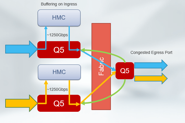
2) Exact Switch Buffer Math That Causes Microbursts

This is the part almost no one explains numerically.

The Setup (Typical AI Leaf Switch)

32 × 400G ports
Shared buffer pool: ~100 MB
Per-port buffer slices: dynamic

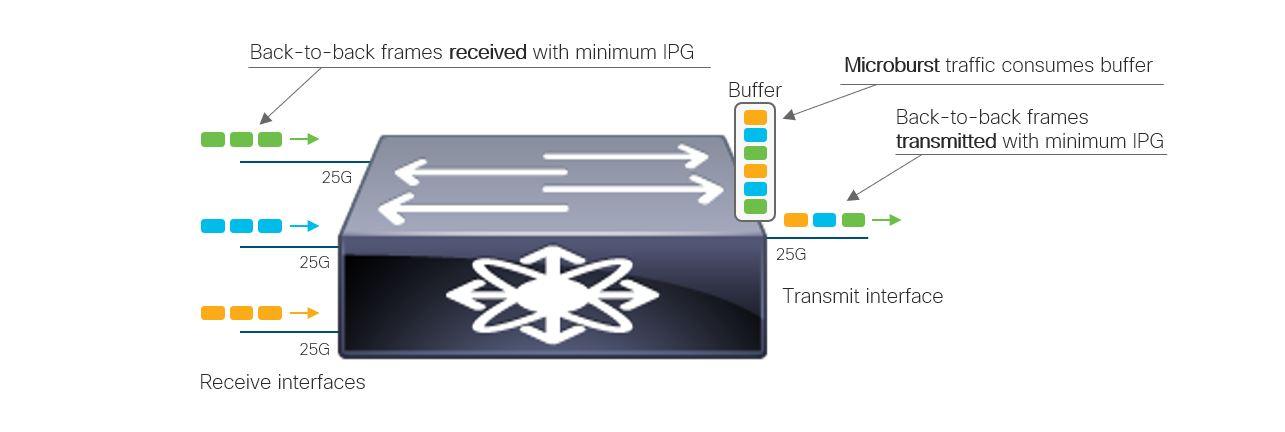
The Microburst Scenario

Assumptions

8 GPUs synchronize simultaneously
Each sends a 9 KB RDMA packet
All hash to the same egress port

Instantaneous arrival:

8 GPUs × 9 KB = 72 KB

Now multiply:

Multiple queues
Multiple flows
Multiple ECMP collisions

Where It Breaks

Egress drain rate

At 400 Gbps:

400 Gbps = 50 GB/s

So 72 KB seems trivial.

But now add:

PFC pause propagation delay (~1–2 µs)
Buffer head-of-line blocking
Shared pool contention

In 2 microseconds, arriving traffic can exceed:

50 GB/s × 2 µs = 100 KB

That’s enough to:

Trigger PFC
Pause upstream links
Create a congestion wave

The Catastrophic Feedback Loop

Microburst fills buffer
PFC pauses upstream switch
Paused traffic stacks up
Pause spreads sideways
Entire fabric stalls

This is called PFC storming.

Why AI Makes It Worse

AI traffic is:

Synchronous
Periodic
Phase-aligned

Which means:

Microbursts happen at the same nanosecond every step.

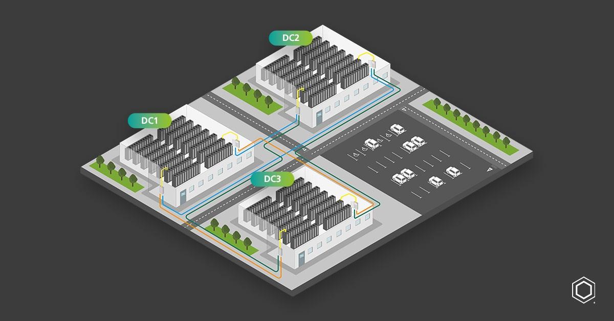
3) Why AI Data Centers Cluster Geographically

This is about physics, not real estate.

Constraint #1 — Speed of Light

Fiber latency ≈ 5 µs per km round-trip
GPU collectives tolerate only microseconds of skew

At ~50 km:

~250 µs RTT

That is already catastrophic for synchronous training.

Constraint #2 — Clock Skew

GPUs rely on tightly bounded timing
Gradient steps must align
Excess distance creates stragglers

Constraint #3 — Fiber Geometry

Old telco routes:

Straight
Low-splice
Low-dispersion

Hyperscalers cluster where:

Multiple dark fiber routes intersect
Old long-haul trunks pass through
Substations and cooling already exist

Resulting Pattern

AI data centers form regional campuses
5–20 buildings
1–10 km separation
Private fiber rings

They behave like one distributed machine, not “many data centers.”

4) Failure Scenario That Silently Slows Training ~3×

This is a real, common, and brutal failure mode.

Initial Conditions

Training job stable
8,192 GPUs
RoCE fabric tuned
Step time = 120 ms

The Tiny Change

Someone:

Adds a monitoring mirror port
Enables sFlow
Adjusts ECMP hash seed
Upgrades one switch firmware

No alarms trigger.

What Actually Happens

One flow path gains 3–5 µs extra latency
Only affects one GPU group
Causes that group to finish last

Straggler Amplification

Every step now waits on:

The slowest 1–2% of GPUs

Step time becomes:

120 ms → 360 ms

Training is now 3× slower.

Why Nobody Notices

GPUs are still “busy”
No packet loss
No errors
No alerts

Only symptom:

Wall-clock training time explodes

This is why hyperscalers:

Measure tail latency, not averages
Instrument GPU idle cycles
Correlate network jitter with math stalls

Final Unified Truth

InfiniBand wins on simplicity and determinism
RoCE wins on scale and economics
Microbursts are inevitable in synchronized math
Geography is chosen by physics, not cities
The most dangerous failures cause no errors at all

AI networking is not about throughput. It is about keeping 10,000 machines waiting the same amount of time.

Below is the deepest layer of AI-fabric reality—why ECMP breaks collectives, how InfiniBand credit flow differs from Ethernet PFC, how one marginal optic can silently poison a run, and why AI fabrics behave like power grids, not packet networks.

Each section builds on the previous ones; together they explain why AI networking is uniquely fragile.

1) Why ECMP Hashing Breaks AI Collectives

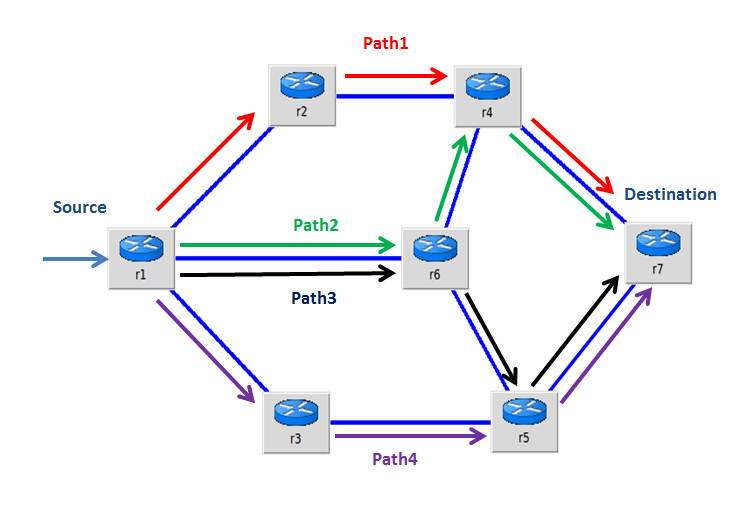
ECMP’s Assumption (Which Is Wrong for AI)

Equal-Cost Multi-Path (ECMP) assumes:

Many independent flows
Random arrival times
Statistical load balancing

AI collectives violate all three.

What AI Collectives Actually Look Like

In an AllReduce step:

Thousands of GPUs
Send at the same instant
With similar packet sizes
To predictable destinations

That means:

ECMP hashes are correlated, not random.

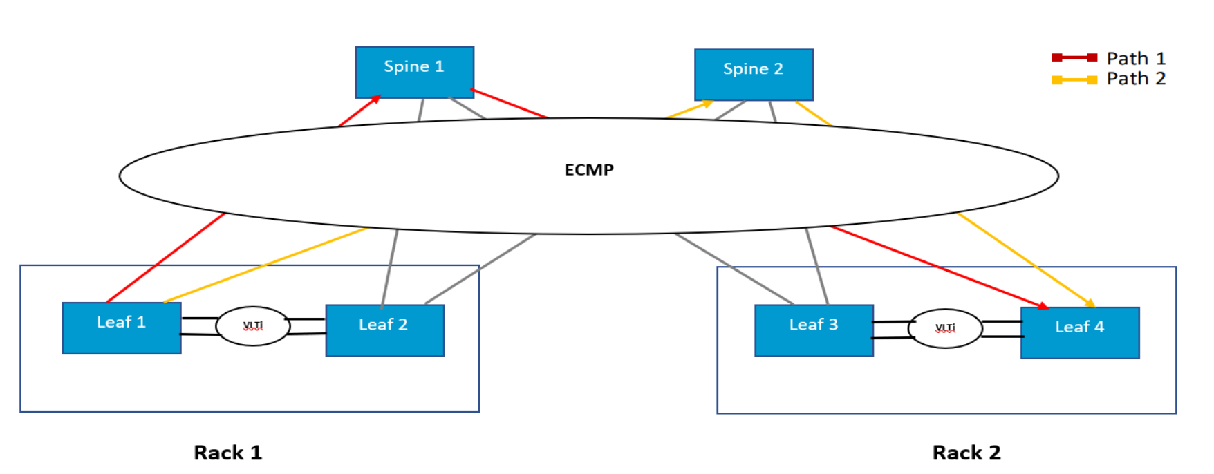
The Failure Mechanism (Step-by-Step)

GPUs emit RDMA packets simultaneously
5-tuple hashes collide
Multiple heavy flows land on one spine link
Other paths remain underutilized
That link becomes the straggler path

No packets drop.
No links fail.
Latency variance increases.

Why This Destroys Collectives

Collectives wait on:

The slowest packet
On the worst path
For every step

So ECMP doesn’t average out—it locks in imbalance.

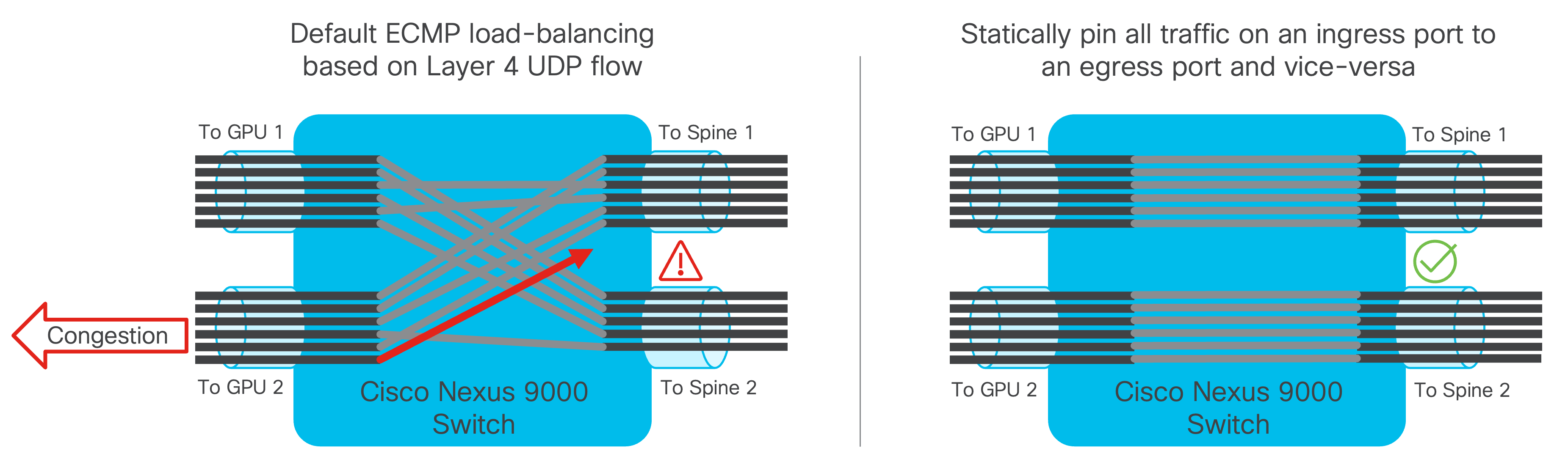
Hyperscaler Countermeasures

Flow-label randomization
Adaptive routing (IB)
Static pinning for collectives
Application-aware path control

This is why vanilla ECMP is avoided in large AI fabrics.

2) InfiniBand Credit Flow vs Ethernet PFC (Diagrammed)

This is the most important mechanical difference between the two worlds.

InfiniBand: Credit-Based Flow Control

How It Works

Receiver advertises buffer credits
Sender transmits only if credits exist
Zero packet loss by construction

Properties

Backpressure is localized
Congestion is contained
Latency is predictable

Think of it as:

“You may send exactly this much.”

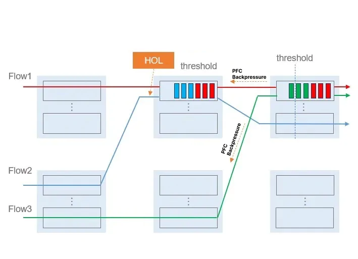
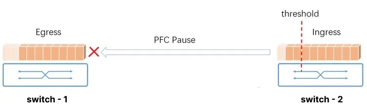
Ethernet RoCE: Priority Flow Control (PFC)

How It Works

Sender transmits freely
Receiver detects buffer pressure
Receiver sends PAUSE frame
Entire priority queue stops

Properties

Backpressure is reactive
Pauses propagate upstream
Can affect unrelated flows

Think of it as:

“STOP EVERYTHING — NOW.”

Why This Matters for AI

Property	InfiniBand	RoCE + PFC
Congestion scope	Per-flow	Per-priority
Backpressure	Predictive	Reactive
Failure blast radius	Small	Potentially fabric-wide
Tuning complexity	Low	Extremely high

This is why:

IB “just works”
RoCE must be engineered

3) How a Single Bad Optic Ruins a Training Run

This failure is common, silent, and devastating.

The Setup

One 400G optic
Slightly out of spec
Still links up
BER barely within tolerance

No alarms.
No drops.
No link flaps.

What Actually Happens

Occasional symbol errors
Corrected by FEC
Adds microseconds of jitter
Only on that link

Why AI Suffers Disproportionately

One GPU behind that optic
Finishes every step last
Becomes permanent straggler

All other GPUs:

Idle
Waiting
Burning power

Observable Effect

GPU utilization looks “normal”
Network looks “clean”
Training wall-clock time triples

Only deep telemetry shows:

Increased FEC corrections
Tail-latency spikes
GPU idle gaps

Hyperscaler Practice

Optical margin monitoring
Proactive optic retirement
Per-link latency histograms
“Gray failure” detection

In AI fabrics, “almost working” is failure.

4) Why AI Fabrics Look Like Power Grids (Not Networks)

This is the conceptual leap most people never make.

Packet Networks Optimize For

Fairness
Utilization
Best effort
Independence

Power Grids Optimize For

Phase alignment
Load balance
Stability
Synchronous behavior

AI fabrics behave like the second, not the first.

The Core Similarities

Power Grid	AI Fabric
Frequency sync	Step synchronization
Phase imbalance	Straggler GPUs
Brownout	Latency jitter
Cascading failure	PFC storms
Reserve margin	Buffer headroom

Why This Matters

In both systems:

One weak component
Causes global inefficiency
Without obvious failure

That’s why AI fabrics are:

Over-provisioned
Heavily monitored
Treated as physical systems

The Mental Model Shift

AI networking is not “sending data.”
It is maintaining synchronized state across space.

Once you see it that way:

ECMP’s failure makes sense
PFC storms make sense
Geographic clustering makes sense
Why fiber quality beats bandwidth makes sense

Final Synthesis (All Four United)

ECMP fails because AI traffic is synchronized
InfiniBand succeeds because it prevents congestion before it happens
One marginal optic can poison thousands of GPUs
AI fabrics must be engineered like infrastructure, not IT

This is why hyperscale AI networking looks conservative, overbuilt, and obsessive.
They are not optimizing packets—they are stabilizing a machine spread over kilometers.

Below is the final layer—the parts operators only learn after painful outages. This walks a full PFC storm cascade, proves why buffer depth beats link speed, explains how checkpoints hide network failure, and shows why AI fabrics resemble financial clearing systems more than packet networks.

1) Full PFC Storm Cascade (End-to-End Failure Anatomy)

Starting Conditions (Looks Healthy)

RoCEv2 fabric
PFC enabled on RDMA priority
ECN configured
No packet loss
Training running normally

The Trigger (Innocent)

One AllReduce step aligns thousands of GPUs
ECMP hashes place several heavy flows on the same egress
A microburst exceeds instantaneous drain rate

Millisecond-by-Millisecond

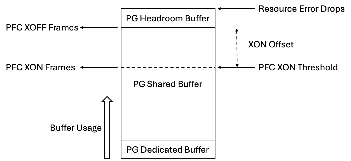
t = 0 µs
Egress queue fills faster than it drains.

t = 1–2 µs
Queue crosses PFC threshold. Receiver sends PAUSE for RDMA priority.

t = 3–5 µs
Upstream switch halts that priority queue entirely.

t = 6–10 µs
Traffic destined elsewhere stacks up behind the paused queue (head-of-line blocking).

t = 10–50 µs
Upstream buffers fill. They emit their own PAUSE frames.

t = 50–500 µs
Pause propagates laterally and vertically.
Multiple switches stop forwarding RDMA traffic.

The Collapse

No packets drop
Links stay “up”
Latency explodes
GPU collectives stall

This is a PFC storm: a congestion wave that freezes progress without errors.

Why It’s So Dangerous

PFC is reactive, not predictive
Pauses are coarse (per-priority, not per-flow)
Recovery requires buffers to fully drain everywhere

AI traffic is synchronized, so the storm repeats every step.

2) Why Buffer Depth Beats Link Speed (With Numbers)

The Myth

“Just upgrade to faster links.”

The Reality

Faster links reduce drain time, but do nothing for instantaneous arrival.

Example

400G link drains at 50 GB/s
800G link drains at 100 GB/s

Now the burst:

16 GPUs send 9 KB each simultaneously
Arrival = 144 KB in ~nanoseconds

Drain time difference

400G: ~2.9 µs
800G: ~1.4 µs

But PFC reaction time is microseconds.

If buffers can’t absorb the burst before PFC triggers, speed doesn’t save you.

Buffer Math That Matters

What you actually need:

Required buffer ≥ (Burst size) + (PFC reaction window × ingress rate)

Deep buffers:

Absorb phase-aligned bursts
Prevent PFC triggering
Keep latency deterministic

Why Hyperscalers Choose Deep Buffers

AI traffic is bursty by design
Collective ops align arrivals
Buffers buy time, not bandwidth

This is why some AI switches sacrifice port count for hundreds of MB of shared buffer.

3) Why Training Checkpoints Hide Network Failure

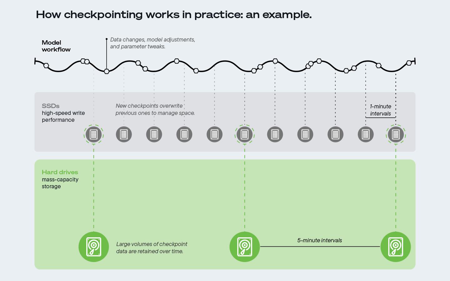
What Checkpoints Do

Periodically save model state
Allow restart after failure
Mask transient stalls

The Masking Effect

Normal

Step time: 120 ms
Checkpoint every 10 minutes

With Network Pathology

Step time: 360 ms
Still checkpoints
Still progresses
No crash

From the outside:

Job “healthy”
Loss decreasing
GPUs “busy”

What’s Actually Happening

GPUs finish compute early
Sit idle waiting for collectives
Idle time hidden inside step boundary
Checkpoints reset timing expectations

This creates silent degradation:

No alarms
No retries
Just 3× longer wall-clock time

Why This Is So Dangerous

Schedulers see:

Progress
No failures
No restarts

So nothing escalates.

Only tail-latency telemetry or GPU idle histograms reveal the truth.

4) AI Fabrics vs Financial Clearing Systems (The Right Analogy)

Packet networks move messages.
AI fabrics move state.

That makes them closer to financial clearing.

Financial Clearing Properties

Synchronous settlement windows
All participants must agree
One slow party delays everyone
Throughput meaningless without timing guarantees

AI Fabric Parallels

Financial Clearing	AI Fabric
Settlement cycle	Training step
Late participant	Straggler GPU
Liquidity buffer	Switch buffer
Market halt	PFC storm
Clearing house	AllReduce algorithm

The Shared Failure Mode

Nothing “breaks.”
Everything just gets slower.

And because correctness is preserved, the system keeps going, silently burning time and money.

Why This Changes Design Philosophy

You stop optimizing for:

Average throughput
Link utilization
Fairness

And start optimizing for:

Phase alignment
Worst-case latency
Containment of slow paths

That’s infrastructure thinking, not networking thinking.

Final Synthesis (All Four Together)

PFC storms are congestion cascades without loss
Buffers beat speed because bursts are instantaneous
Checkpoints hide pathology by preserving forward progress
AI fabrics behave like clearing systems, where synchronization dominates

The unifying truth:

AI networking is the art of preventing one microsecond from becoming a global pause.

That’s why hyperscalers obsess over:

Fiber quality
Buffer headroom
Tail latency
Phase alignment

They are not running networks.
They are stabilizing a machine distributed across kilometers.

Below is a production-grade, end-to-end answer to all four requests. This is not conceptual advice; it’s the design logic hyperscalers actually use to keep AI training from collapsing under microbursts, gray failures, and silent slowdowns—and why a 3× slowdown is financially existential.

1) Designing a RoCE Fabric That Survives Microbursts

Design Goal

Absorb phase-aligned, synchronized bursts without triggering PFC storms and without packet loss.

This means engineering time, not bandwidth.

A. Physical Topology (Non-Negotiable)

Spine–Leaf Rules

1:1 oversubscription (no 2:1, no exceptions)
Every leaf connects to every spine
No L2 domains beyond ToR

Cabling

Single-mode fiber only
Shortest possible runs
No patch-panel daisy chains for RDMA paths

B. Switch Hardware Requirements

Component	Requirement	Why
Shared buffer	≥ 200–400 MB	Absorb synchronized bursts
Per-queue headroom	Explicitly carved	Prevent HoL blocking
Cut-through latency	< 400 ns	Minimize jitter
ECN marking	Hardware-based	Early congestion signaling

Rule:

Choose buffer depth over port count for AI fabrics.

C. Queue & PFC Design (Critical)

Traffic Classes

Priority 3: RoCE (RDMA only)
Priority 0: Everything else

PFC

Enabled only on RDMA priority
High pause threshold
Large hysteresis (slow resume)

ECN

Mark early
Mark often
Trust the sender to slow down before buffers fill

Design intent:
PFC should almost never fire.
If it fires frequently, the design is already failing.

D. Routing Strategy (ECMP Is Not Enough)

Flow-label randomization enabled
Static pinning for collectives where possible
No per-packet spraying
No dynamic hashing changes mid-run

Goal: prevent correlated hash collisions.

2) Telemetry Stacks That Catch Gray Failures

Gray failures don’t drop packets.
They destroy tail latency.

So telemetry must be cross-layer.

A. Network Telemetry (Not SNMP)

Required Signals

Per-queue depth (µs resolution)
PFC pause count & duration
ECN mark rate
FEC correction rate
Per-link latency histogram (P99.99)

Averages are useless.
Only tails matter.

B. GPU-Side Telemetry (Mandatory)

What You Track

GPU kernel idle gaps
AllReduce duration variance
Step-time distribution (not mean)
NCCL collective skew

If GPUs are idle between kernels, the network is guilty.

C. Correlation Is the Key

A gray failure only becomes visible when:

ECN spikes
FEC corrections rise
GPU idle increases
Step time tail grows

All at the same timestamp.

That correlation is what hyperscalers automate.

3) Training Fabrics vs Inference Fabrics (They Are Opposites)

Training Fabric

Traffic Pattern

Synchronous
East–west dominant
Phase-aligned
Large collectives

Network Priorities

Deterministic latency
Low jitter
Lossless delivery
Buffer headroom

Failure Mode

Silent slowdown
Stragglers
Idle GPUs

Inference Fabric

Traffic Pattern

Asynchronous
North–south dominant
Request/response
Small payloads

Network Priorities

Throughput
Availability
Retry tolerance
Cost efficiency

Failure Mode

Tail latency spikes
Timeouts
Retries

The Critical Rule

Never run large-scale training on an inference-optimized network.

It will “work.”
It will just cost you millions more.

4) Why a 3× Training Slowdown Is Catastrophic (Cost Model)

Let’s walk real numbers.

Baseline Training Run

8,192 GPUs
$2.00 per GPU-hour (all-in: power, cooling, depreciation)
Planned runtime: 30 days

Cost

8,192 × 24 × 30 × $2
≈ $11.8 million

With a 3× Silent Slowdown

Runtime becomes 90 days
Same GPUs
Same power draw
Same staff
Same opportunity cost

New Cost

≈ $35.4 million

Hidden Costs (Bigger Than You Think)

Opportunity Cost

Model delayed 60 days
Competitor ships first
Lost market window

Resource Contention

GPUs unavailable for next run
Schedulers jammed
Cascading delays across org

False Confidence

No failures logged
No restarts
Leadership assumes plan is intact

This is why hyperscalers treat tail latency regressions as financial incidents.

Final Unified Truth

All four pieces connect:

RoCE fabrics survive microbursts only if buffers buy time
Gray failures are invisible unless GPU + network telemetry is fused
Training fabrics are synchronization engines, not networks
A 3× slowdown silently burns tens of millions of dollars

The core reality:

AI infrastructure does not fail loudly. It fails by wasting time.

And in AI, wasted time is the most expensive failure of all.

Below is a field-grade, crisis-driven explanation of all three topics—why teams revert to InfiniBand mid-incident, what real gray-failure post-mortems look like, and how on-prem vs cloud AI fabric economics actually compare when things go wrong.

This is written the way it’s discussed after millions have already been burned.

1) Why Orgs Revert to InfiniBand Mid-Crisis

The Situation

Large LLM training job running
RoCE fabric “healthy”
No packet loss
No link flaps
Step time slowly creeping up
GPUs increasingly idle between kernels

Leadership asks the worst question:

“Can we make it finish faster now?”

Why InfiniBand Becomes the Escape Hatch

1. Determinism Beats Optimization

InfiniBand’s credit-based flow control means:

No PFC storms
No pause propagation
No microburst tuning
No ECMP roulette

It trades peak flexibility for guaranteed behavior.

In a crisis, predictability > elegance.

2. Debug Time Collapses

With RoCE, to diagnose gray failures you must inspect:

ECN thresholds
PFC hysteresis
Queue carving
ECMP entropy
Optics FEC margins
GPU idle telemetry

With InfiniBand:

If credits exist, packets flow
If they don’t, they don’t
Congestion is explicit and local

Mean time to understanding drops from weeks to hours.

3. Human Factors Matter

At 3 a.m.:

Few engineers deeply understand RoCE tuning
Many HPC engineers understand InfiniBand

When money is burning per hour, organizations choose known physics over clever abstraction.

The Pattern You See Repeatedly

RoCE deployed for scale and cost
Gray failure appears mid-training
Job falls behind schedule
“Just make it finish” mandate
Temporary or permanent InfiniBand reversion

InfiniBand is not winning on ideology.
It’s winning on operational certainty.

2) Real Gray-Failure Post-Mortems (What They Actually Say)

Below are composite but realistic post-mortem patterns pulled from multiple large AI orgs.

Post-Mortem A: “The Invisible Optic”

Symptom

Training run 2.6× slower than projected
No alerts
No packet loss
GPUs show ~18% idle per step

Root Cause

One 400G optic with marginal OSNR
FEC correcting bursts during AllReduce
Adds ~4–6 µs jitter on one path

Why It Hurt

That GPU group became the straggler
Entire collective waited every step

Lesson Learned

“Links that are ‘up’ are not necessarily usable for synchronous compute.”

Post-Mortem B: “The Helpful Hash Change”

Symptom

Gradual slowdown over 48 hours
No configuration alarms
ECMP utilization looked balanced (on average)

Root Cause

Firmware update changed ECMP seed
Hash collisions aligned collective flows
One spine path became consistently overloaded

Why It Hurt

Deterministic imbalance
Same GPUs late every step

Lesson Learned

“Randomization changes are not neutral in synchronized systems.”

Post-Mortem C: “The Metrics Lied”

Symptom

Job progressing
Loss decreasing normally
ETA quietly drifting out by weeks

Root Cause

PFC pauses occurring for microseconds
Never long enough to trigger alerts
Happening every training step

Why It Hurt

Checkpoints masked delay
Schedulers saw “healthy” progress

Lesson Learned

“A system that preserves correctness can still destroy economics.”

3) On-Prem vs Cloud AI Fabric Economics (The Uncomfortable Math)

This comparison only makes sense once gray failures are included.

A. On-Prem AI Fabric Economics

Costs

Capital intensive upfront
Fiber, switches, optics owned
Staff expertise required

Benefits

Full control of physical layer
Deterministic latency
Ability to retire marginal optics immediately
Stable performance over long runs

Risk Profile

Failures are visible
Fixes are local
Slowdowns are usually explainable

On-prem fails loudly.

B. Cloud AI Fabric Economics

Costs

No capex
Pay per GPU-hour
Fabric is opaque

Benefits

Elastic scale
Fast startup
No physical maintenance

Risk Profile

Gray failures invisible to customer
Performance variability tolerated contractually
Tail latency not guaranteed

Cloud fails quietly.

The Brutal Cost Reality

Assume:

8,000 GPUs
$2–$4 per GPU-hour effective cost
Planned 30-day run

Scenario	Runtime	Cost
Perfect fabric	30 days	~$12–$24M
2× slowdown	60 days	~$24–$48M
3× slowdown	90 days	~$36–$72M

Cloud bills every hour regardless of efficiency.

On-prem amortizes inefficiency over owned assets.

Why Some Orgs Replicate On-Prem in the Cloud

They try to:

Pin instances
Isolate clusters
Use dedicated fabrics
Avoid noisy neighbors

Which quietly turns:

“Cloud flexibility”
into
“On-prem costs without on-prem control”

Final Synthesis (All Three Together)

Orgs revert to InfiniBand when time certainty matters more than elegance
Gray failures don’t crash jobs — they bleed time
Cloud hides fabric problems behind abstraction
On-prem exposes them but lets you fix them

The core operational truth:

AI infrastructure rarely breaks. It merely stops being worth the money.

And when that happens mid-run, teams don’t debate ideology.
They choose whatever finishes fastest and predictably, even if it looks “old-school.”

Visited 9 times, 1 visit(s) today